Pythonによるフォルマント分析と音声認識
今回,株式会社サイシードのインターンシップで音声認識の仕組みを学び,音声認識システムをゼロから作るということにチャレンジしてみました.
この記事では音声認識に関する基本的な仕組みを実際に実装し,母音をクラス分類した結果までの一連の流れを書きます.
目次
- 音声認識の仕組み
- Julius
- フォルマント
- フォルマント分析とは
- 母音のフォルマントの抽出に関する実装
- フォルマントを用いた母音のクラス分類
- k近傍法による母音のクラス分類
- SVMによる母音のクラス分類
- 考察
- まとめ
- 参考
音声認識の仕組み
音声認識では連続的な音声を認識する場合,音響モデルと言語モデルを用意します.
音響モデルは音声波形から音素の音響的特徴を求め,各単語の標準のパターンを作成します.
言語モデルはそれぞれの単語間・音素間のつながりを統計的に処理を行い,もっともらしい文章や単語列を生成します.
音声認識ではこの二つのモデルを用いて音素から単語を予測し,単語から文章の繋がりを予測していきます.
今回は,音響モデルの中で音素の特徴を求める手法の一つであるLPC分析を行い,母音のフォルマント抽出とその分類に挑戦していきます.
ちなみに
今回,音素抽出にはJuliusを用いています.
Juliusは音声認識システムの開発・研究のためのオープンソースの音声認識エンジンです.
音声認識はGoogleやIBM,Microsoftなどで試すことができますが無料で行うには制限があります. そういった面で,Juliusでは音声認識に触れてみたい人にとってオススメの音声認識エンジンとなっています.
Julius自体は音声認識エンジンであり,別途音響モデルや単語辞書,言語モデルが必要となりますが,そちらに関しても標準のモデルが提供されています.
フォルマントとは
人の音声は声帯の振動で生成され,声道を通り,口唇から発せられます.その声道には複数の共鳴周波数があり,特定の周波数の音声が強くなります.この強くなった周波数をフォルマント周波数と呼びます.フォルマント周波数は低いものから順に,第一フォルマント(F1),第二フォルマント(F2),・・・と呼ばれ,母音を特徴づけるのに大きく関わっています.
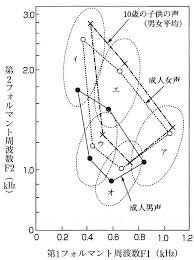
『英語リスニング科学的上達法』の148ページ
今回は文章を読み上げた音声データから音素を抽出し,母音の音素に関してフォルマント分析していきます.
母音のフォルマントの抽出に関する実装
まず,集めた音声データをJuliusのsegmentation-kitを用いて音声データを音素に分割します.分割する際に,音声データに対応するテキストデータを用意し,segment_julius.plを実行すると以下のようなlabファイルが作成されます.
    0.0000000 0.6325000 silB
    0.6325000 0.7025000 s
    0.7025000 0.8225000 e
    0.8225000 0.8925000 ts
    0.8925000 0.9525000 u
    0.9525000 1.0125000 m
    1.0125000 1.1425000 e
    1.1425000 1.1825000 i
    1.1825000 1.2325000 k
    1.2325000 1.3325000 a
    1.3325000 1.3725000 i
    1.3725000 2.0075000 silE
※Juliusではサンプリング周波数16kHz,量子化ビット数16ビット固定,チャンネル数1チャンネル(モノラル)の音声データ(wav形式)に対応しているのでffmpegなどで変換してください.(コードは以下のようにすれば整えられます.)
$ ffmpeg -i input.wav -ac 1 -ar 16000 -acodec pcm_s16le output.wav
次に,segmentation-kitによって得られた各音素の発声タイミングのデータを使い,音声データを切り出し,音素波形を確認します.
phoneme_img.py
    # 使用するパッケージ
    import matplotlib.pyplot as plt
    import cis
    from collections import defaultdict

    #音素部分の画像出力
    for i in range(1,100,1):
        data_list = []
        open_file = "lab_and_text/sound-"+str(i).zfill(3)+".lab"
        filename = "wav/sound-"+str(i).zfill(3)
        v ,fs = cis.wavread(filename+".wav")
        #labファイルの音素データに関する情報を格納
        with open(open_file,"r") as f:
            data = f.readline().split()
            while data:
                data_list.append(data)
                data = f.readline().split()
            #各音素毎に保存したいので,alphabetの辞書を作成
            saisei_dic = defaultdict(list)
            #音素ラベル,開始・終了タイミングを辞書に追加
            for j in range(len(data_list)):
                label =  data_list[j][2]
                if label != "silB" and label != "silE":
                    x1 = int(fs * float(data_list[j][0]))
                    x2 = int(fs * float(data_list[j][1]))
                    saisei_dic[label].append([x1, x2])
            #音素の波形画像を出力
            for j in saisei_dic:
                for k in range(len(saisei_dic[j])):
                    fig = plt.figure()
                    ax = fig.add_subplot(1, 1, 1)
                    ax.plot(v[saisei_dic[j][k][0]:saisei_dic[j][k][1]])
                    plt.savefig('Phoneme_file/' + j + '_' + str(i) + '_' + str(k) + '.png')
得られた音素波形は以下のようになっています.(x軸,y軸のスケールは調整していません.)
母音(/a/)に関してうまく出ていると以下のような画像が出力されます.
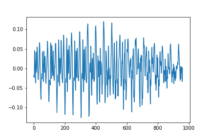
図1.母音aの音声波形
子音(/b/)に関しては以下のような画像が出力されます.
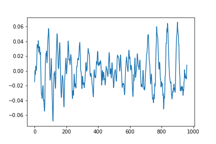
図2.子音bの音声波形
次に,母音の音素に対してフォルマントを求め,線形予測分析(LPC)を使ってフォルマントの包絡とそのピークを抽出していきます.
formant_analysis.py
    #使用するパッケージ
    import cis
    import numpy as np
    import scipy.signal
    from levinson_durbin import autocorr, LevinsonDurbin
    from collections import defaultdict
    import matplotlib.pyplot as plt
    from scipy.fftpack import fft

    #プリエンファシス(高域強調)
    def preEmphasis(wave, p=0.97):
        # 係数 (1.0, -p) のFIRフィルタを作成
        return scipy.signal.lfilter([1.0, -p], 1, wave)

    boin_list = ["a","i","u","e","o"]

    #データの読み込み, 音素ごとに辞書化
    for i in range(1,100,1):
        data_list = []
        open_file = "lab_and_text/sound-"+str(i).zfill(3)+".lab"
        filename = "wav/sound-"+str(i).zfill(3)
        v ,fs = cis.wavread(filename+".wav")
        with open(open_file,"r") as f:
            data = f.readline().split()
            while data:
                data_list.append(data)
                data = f.readline().split()
            saisei_dic = defaultdict(list)
            for j in range(len(data_list)):
                label =  data_list[j][2]
                if label in boin_list:
                    x1 = int(fs * float(data_list[j][0]))
                    x2 = int(fs * float(data_list[j][1]))
                    saisei_dic[label].append([x1, x2])
            for j in saisei_dic:
                for k in range(len(saisei_dic[j])):
                    # LPC係数を求める(lpcの次数は要調整)
                    lpcOrder = 16
                    #短すぎるデータは扱いづらいので削除
                    start = saisei_dic[j][k][0]
                    end = saisei_dic[j][k][1]
                    if (end - start) <= fs//200:
                        continue
                    fig = plt.figure()
                    ax = fig.add_subplot(1, 1, 1)
                    #センター部分を使う
                    center = (end + start) // 2
                    cuttime = 0.04
                    voice_data = v[center - int(cuttime / 2 * fs) : center + int(cuttime / 2 * fs)]
                    #正規化
                    voice_data = voice_data/max(abs(voice_data))
                    #プリエンファシス
                    p = 0.97
                    voice_data = preEmphasis(voice_data, p)
                    #ハミング窓
                    hammingWindow = np.hamming(len(voice_data))
                    voice_data = voice_data * hammingWindow
                    r = autocorr(voice_data, lpcOrder + 1)
                    a, e  = LevinsonDurbin(r, lpcOrder)
                    # LPC係数の振幅スペクトルを求める
                    sample = len(voice_data)
                    fscale = np.fft.fftfreq(sample, d = 1.0 / fs)[:sample//2]
                    # オリジナル信号の対数スペクトル
                    spec = np.abs(fft(voice_data, sample))
                    logspec = 20 * np.log10(spec)
                    ax.plot(fscale, logspec[:sample//2])
                    # LPC対数スペクトル
                    w, h = scipy.signal.freqz(np.sqrt(e), a, sample, "whole")
                    lpcspec = np.abs(h)
                    loglpcspec = 20 * np.log10(lpcspec)
                    #出力をプロットしてみて出力
                    ax.plot(fscale, loglpcspec[:sample//2], "r", linewidth=2)
                    maxId = scipy.signal.argrelmax(loglpcspec[:sample//2],order=3)
                    maxId = maxId[0]
                    #とりあえず4つ分ぐらいのフォルマントの位置を出力
                    ax.axvline(fscale[maxId[0]], ls = "--", color = "navy")
                    ax.axvline(fscale[maxId[1]], ls = "--", color = "navy")
                    ax.axvline(fscale[maxId[2]], ls = "--", color = "navy")
                    ax.axvline(fscale[maxId[3]], ls = "--", color = "navy")
                    plt.savefig('formant_file/'+j+'_'+str(i)+'_'+str(k)+'.png')
例えば,図1の母音aのフォルマントは次のように出力されます.
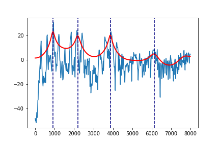
図3.図1の母音aの波形の包絡
また,本プログラムで利用したlevinson_durbin,LPCは人工知能に関する断創録さんのプログラムを参考にしています.
全てのデータ(5000程度)の第1,第2フォルマントをplotした結果は次のようになります.
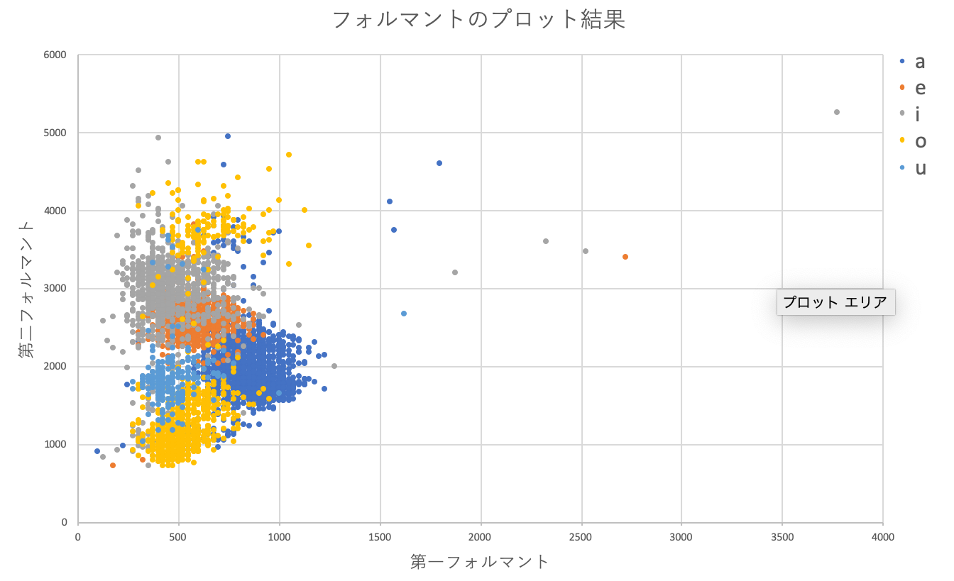
図4.フォルマントのプロット結果
明らかな外れ値もありますが,パッと見6分類ぐらいでいけそうな・・・
とりあえず分類してみましょう.
k近傍法による母音のクラス分類
まずはkNNを試していきます.
knn.py
    #k-近傍法
    import matplotlib.pyplot as plt
    import pandas as pd
    from sklearn.neighbors import KNeighborsClassifier as KNN

    #データセットの読み込み
    formant_df = pd.read_csv("formant5.csv", encoding="shift-jis")

    # データのシャッフル
    formant_df = formant_df.sample(frac = 1).reset_index(drop=True)
    #教師データとテストデータの境目を決める
    use_row_limit = int(formant_df.shape[0] * 0.8)
    use_column = list(range(formant_df.shape[1]))[1:]
    train_data = formant_df.iloc[:use_row_limit,:]
    test_data = formant_df.iloc[use_row_limit:,:]

    list_nn = []
    list_score = []
    max_score = 0
    for k in range(1,50):
        knn = KNN(n_neighbors = k,n_jobs = -1)

        knn.fit(
            train_data.iloc[:,use_column].values,
            train_data["vowel"].values,
        )

        pred_target = knn.predict(
            test_data.iloc[:,use_column].values
        )
        list_nn.append(k)
        score = sum(test_data["vowel"] == pred_target) / len(pred_target)
        list_score.append(score)
        if score >= max_score:
            max_score = score
    #プロット
    plt.ylim(0.75, 0.90)
    plt.xlabel("n_neighbors")
    plt.ylabel("score")
    plt.plot(list_nn, list_score)
    print(max_score)
今回k=1~50で回してみた結果一番いい精度は
0.852112676056338
プロット結果は以下のようになっています.
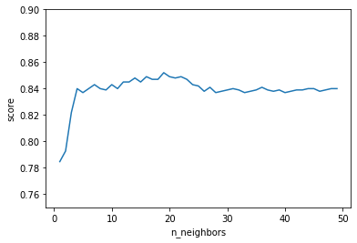
図5. kNNの精度
元の状態から考えるとなかなかいい精度で分類できてそうです.
SVMによる母音のクラス分類
続いて,SVMでクラス分類してみます.
カーネルが簡単に選択できるので,とりあえず3つほど試してみます.
svm.py
    #SVM
    #必要なパッケージ
    import numpy as np
    import pandas as pd
    from sklearn.model_selection import train_test_split
    from sklearn.preprocessing import StandardScaler
    from sklearn.svm import SVC
    from sklearn.metrics import accuracy_score

    #データセットの読み込み
    formant_df = pd.read_csv("formant5.csv", encoding="shift-jis")

    # データのシャッフル
    formant_df = formant_df.sample(frac = 1).reset_index(drop=True)
    x = formant_df.iloc[:, [1,2]]#F1とF2
    y = formant_df.iloc[:, 0]#a,i,u,e,oのラベル

    #ラベルは一旦数字に変更
    y[y == "a"] = 0
    y[y == "i"] = 1
    y[y == "u"] = 2
    y[y == "e"] = 3
    y[y == "o"] = 4
    y = np.array(y, dtype = "int")

    #教師データとテストデータの境目を決める
    x_train, x_test, y_train, y_test = train_test_split(x, y, test_size = 0.3, random_state = None)

    #データの標準化
    sc = StandardScaler()
    sc.fit(x_train)
    x_train_std = sc.transform(x_train)
    x_test_std = sc.transform(x_test)

    #SVMのインスタンスを生成
    model_linear = SVC(kernel = 'linear', random_state = None)
    model_poly = SVC(kernel = "poly")
    model_rbf = SVC(kernel = "rbf")
    model_linear.fit(x_train_std, y_train)
    model_poly.fit(x_train_std, y_train)
    model_rbf.fit(x_train_std, y_train)

    pred_linear_train = model_linear.predict(x_train_std)
    pred_poly_train = model_poly.predict(x_train_std)
    pred_rbf_train = model_rbf.predict(x_train_std)
    accuracy_linear_train = accuracy_score(y_train, pred_linear_train)
    accuracy_poly_train = accuracy_score(y_train, pred_poly_train)
    accuracy_rbf_train = accuracy_score(y_train, pred_rbf_train)
    print("train_result")
    print("Linear : " + str(accuracy_linear_train))
    print("Poly : " + str(accuracy_poly_train))
    print("RBF : " + str(accuracy_rbf_train))

    pred_linear_test = model_linear.predict(x_test_std)
    pred_poly_test = model_poly.predict(x_test_std)
    pred_rbf_test = model_rbf.predict(x_test_std)
    accuracy_linear_test = accuracy_score(y_test, pred_linear_test)
    accuracy_poly_test = accuracy_score(y_test, pred_poly_test)
    accuracy_rbf_test = accuracy_score(y_test, pred_rbf_test)
    print("-" * 40)
    print("test_result")
    print("Linear : " + str(accuracy_linear_test))
    print("Poly : " + str(accuracy_poly_test))
    print("RBF : " + str(accuracy_rbf_test))
実行した結果は次のようになります.
    train_result
    Linear : 0.8109896432681243
    Poly : 0.7206559263521288
    RBF : 0.8550057537399309
    ----------------------------------------
    test_result
    Linear : 0.7825503355704698
    Poly : 0.6932885906040268
    RBF : 0.8308724832214766
今回のデータにはRBFを指定したほうがよさそうですね.
次元数が多くなってきたら,Linearを使うといいそうです.
また,kernelは指定なしでは通常RBFが指定されます.
中身がどうなっているのかよくわからないので図にプロットしてみます.
plot_svm_result.py
    import matplotlib.pyplot as plt
    from mlxtend.plotting import plot_decision_regions
    plt.style.use('ggplot')

    X_combined_std = np.vstack((x_train_std, x_test_std))
    X_combined_std
    y_combined = np.hstack((y_train, y_test))

    fig = plt.figure(figsize = (13,8))
    plot_decision_regions(X_combined_std, y_combined, clf = model_linear)
    plt.show()
    fig = plt.figure(figsize = (13,8))
    plot_decision_regions(X_combined_std, y_combined, clf = model_poly)
    plt.show()
    fig = plt.figure(figsize = (13,8))
    plot_decision_regions(X_combined_std, y_combined, clf = model_rbf)
    plt.show()
プログラムはKazuki
Hayakawaさんの記事に詳しく記載されています.
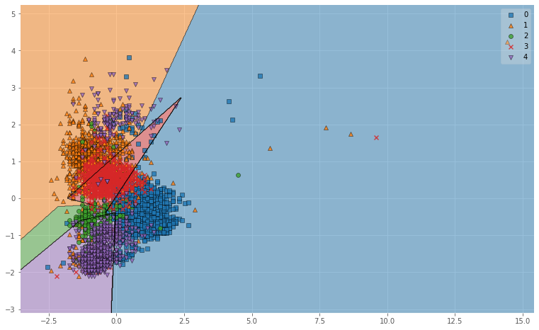
図6. Linearによる母音の分類結果(※0:a, 1:i, 2:u, 3:e, 4:o)
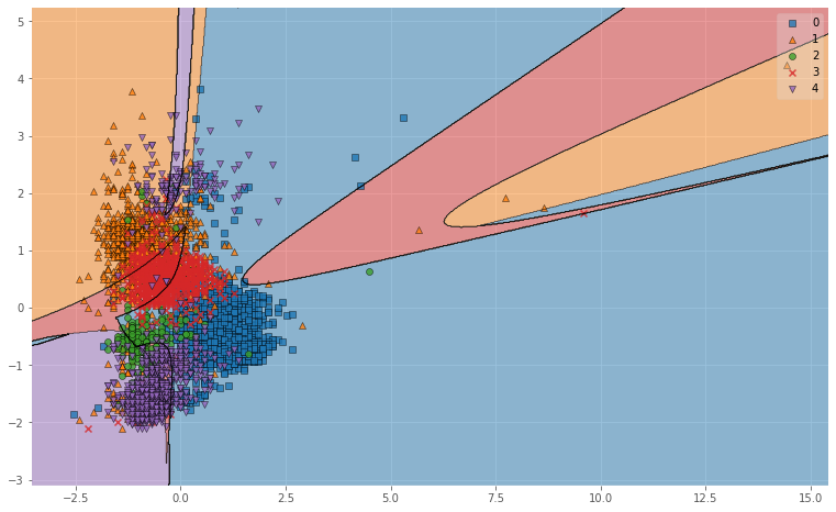
図6. Polyによる母音の分類結果(※0:a, 1:i, 2:u, 3:e, 4:o)
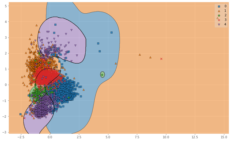
図6. RBFによる母音の分類結果(※0:a, 1:i, 2:u, 3:e, 4:o)
図示してみるとRBFがよかった理由がわかりやすいですね.
RBFはデータを非線形空間(ガウス関数)に変換し,複雑なデータ群をよりシンプルに捉えることができるので,
単純に線引きをするよりも精度が上がります.
考察
音声データからの音素抽出・音素のフォルマント分析・母音のクラス分類という基本的な音声認識の流れをプログラムを作りながら,追ってみました.
今回,音声認識データの母音分類結果としては83%前後の精度を得ることができました.
これは用いた音声データが一人の音声から集められているものなのでこのような結果を得ることができたと考えられます.たくさんの人の音声を集めて同じことをやると精度は落ちていくことが考えられます.
一方で,音素のセグメンテーションでは日本語訳と音声の不一致や音素抽出部分のずれなどの影響により母音の単音発声と比べるとノイズの多いものとなっています.これらの影響でうまくフォルマント分析することができていないデータ群が存在していることが考えられ,それが認識精度の減少に繋がっていると思います.
実環境で応用していくには,ある程度の長文音声データにも対応する必要があります.そのためには,より正確な音素セグメンテーションとより高い精度の分析手法が求められます.
今後はそれらの分析手法に関しても実装していきたいと考えています.
まとめ
本記事では音声データを音素に分解するところから実際に母音をフォルマント分析してみるまでを書いてみました.
部分部分に関しては詳しく書いてある記事があると思いますが,実際にゼロベースから分類までを記載している記事というのは少ないと思います.
音声認識の分析を過程への理解したい方,とりあえず試してみたいという方のための記事になれば幸いです.
今後はMFCCなどを用いてより本格的な音声認識を実装していきたいと思います.
追記
MFCCに関する記事をあげましたのでそちらもよければご覧ください.(2019/12/13)
参考
- 人工知能に関する断創録
- Kazuki Hayakawaさんの記事
- 音声認識(MLPシリーズ)
- Pythonで学ぶ実践画像・音声処理入門